图像二值化

1. 理论

图像的二值化，就是将图像上的像素点的灰度值设置为0或255，也就是将整个图像呈现出明显的只有黑和白的视觉效果。

一幅图像包括目标物体、背景还有噪声，要想从多值的数字图像中直接提取出目标物体，常用的方法就是设定一个阈值T，用T将图像的数据分成两部分：大于T的像素群和小于T的像素群。这是研究灰度变换的最特殊的方法，称为图像的二值化（Binarization）。

常见的二值化方法有三种，分别是固定阈值法、平均值法、自适应阈值法和直方图法。

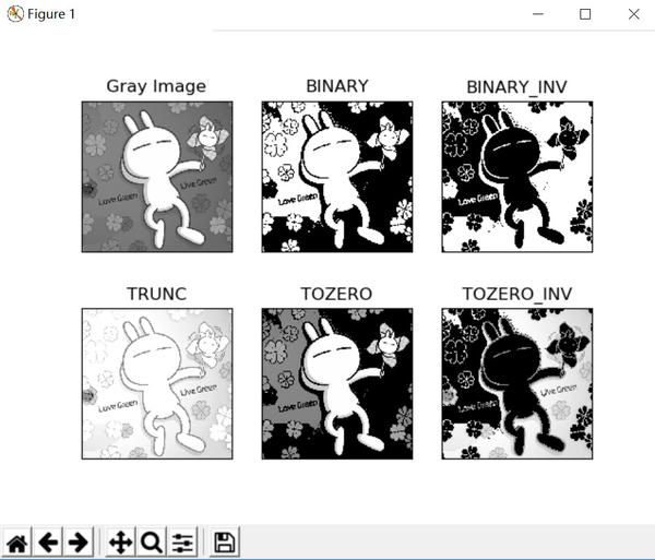
固定阈值法就是设定一个固定阈值K，小于等于K的像素值设为0(黑色)，大于K的像素值设为255(白色)。

平均值法计算像素的平均值K，然后扫描图像的每个像素值，小于等于K像素值设为0(黑色)，大于K的像素值设为255(白色)。

自适应阈值法对平均值法进行改进，规定一个区域大小，求区域平均值作为阈值K，然后区域中的像素值与K进行比较。

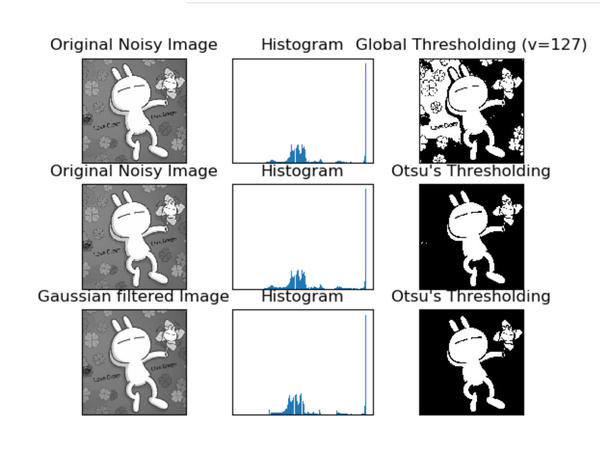
直方图方法主要是发现图像的两个最高的峰，然后阈值K取值在两个峰之间的峰谷最低处。图像的直方图用来表征该图像像素值的分布情况。用一定数目的小区间(bin)来指定表征像素值的范围，每个小区间会得到落入该小区间表示范围的像素数目。

更多内容参考图像的二值化之python+opencv和opencv python图像二值化。

2. 实践

2.1. 固定阈值法

import cv2
from matplotlib import pyplot as plt
img=cv2.imread('../image/test.jpg')
GrayImage=cv2.cvtColor(img,cv2.COLOR_BGR2GRAY)
ret,thresh1=cv2.threshold(GrayImage,127,255,cv2.THRESH_BINARY)
ret,thresh2=cv2.threshold(GrayImage,127,255,cv2.THRESH_BINARY_INV)
ret,thresh3=cv2.threshold(GrayImage,127,255,cv2.THRESH_TRUNC)
ret,thresh4=cv2.threshold(GrayImage,127,255,cv2.THRESH_TOZERO)
ret,thresh5=cv2.threshold(GrayImage,127,255,cv2.THRESH_TOZERO_INV)
titles = ['Gray Image','BINARY','BINARY_INV','TRUNC','TOZERO','TOZERO_INV']
images = [GrayImage, thresh1, thresh2, thresh3, thresh4, thresh5]
for i in range(6):
   plt.subplot(2,3,i+1),plt.imshow(images[i],'gray')
   plt.title(titles[i])
   plt.xticks([]),plt.yticks([])
plt.show()

如果报错没有matplotlib，那么先执行pip install matplotlib进行安装。

retval,dst = cv.threshold(src, thresh, maxval, type[, dst] )参数解释：

• src：原图像，原图像应该是灰度图。
• thresh：用来对像素值进行分类的阈值。
• maxval：大于阈值置为maxval。
• type：不同的阈值方法。

2.2. 平均阈值法

import cv2
import numpy as np
from matplotlib import pyplot as plt
img=cv2.imread('../image/test.jpg')
GrayImage=cv2.cvtColor(img,cv2.COLOR_BGR2GRAY)
k=np.mean(GrayImage)
ret,thresh1=cv2.threshold(GrayImage,k,255,cv2.THRESH_BINARY)
ret,thresh2=cv2.threshold(GrayImage,k,255,cv2.THRESH_BINARY_INV)
ret,thresh3=cv2.threshold(GrayImage,k,255,cv2.THRESH_TRUNC)
ret,thresh4=cv2.threshold(GrayImage,k,255,cv2.THRESH_TOZERO)
ret,thresh5=cv2.threshold(GrayImage,k,255,cv2.THRESH_TOZERO_INV)
titles = ['Gray Image','BINARY','BINARY_INV','TRUNC','TOZERO','TOZERO_INV']
images = [GrayImage, thresh1, thresh2, thresh3, thresh4, thresh5]
for i in range(6):
   plt.subplot(2,3,i+1),plt.imshow(images[i],'gray')
   plt.title(titles[i])
   plt.xticks([]),plt.yticks([])
plt.show()

2.3. 自适应阈值法

import cv2
from matplotlib import pyplot as plt
img=cv2.imread('../image/test.jpg')
GrayImage=cv2.cvtColor(img,cv2.COLOR_BGR2GRAY)
ret,th1 = cv2.threshold(GrayImage,127,255,cv2.THRESH_BINARY)

th2 = cv2.adaptiveThreshold(GrayImage,255,cv2.ADAPTIVE_THRESH_MEAN_C,\
                    cv2.THRESH_BINARY,3,4)
th3 = cv2.adaptiveThreshold(GrayImage,255,cv2.ADAPTIVE_THRESH_GAUSSIAN_C,\
                    cv2.THRESH_BINARY,3,4)
titles = ['Gray Image', 'Global Thresholding (v = 127)',
'Adaptive Mean Thresholding', 'Adaptive Gaussian Thresholding']
images = [GrayImage, th1, th2, th3]
for i in range(4):
   plt.subplot(2,2,i+1),plt.imshow(images[i],'gray')
   plt.title(titles[i])
   plt.xticks([]),plt.yticks([])
plt.show()

dst = cv.adaptiveThreshold(src, maxValue, adaptiveMethod, thresholdType, blockSize, C[, dst] )参数解释：

• src：指原图像，原图像应该是灰度图。
• maxValue：大于阈值置为maxValue。
• adaptiveMethod：要使用的自适应阈值算法。
• thresholdType：阈值类型必须是THRESH_BINARY或THRESH_BINARY_INV。
• blockSize：用于计算像素的阈值的像素邻域的大小：3,5,7等。
• C：从平均值或加权平均值中减去常数。通常情况下，它是正数，但也可能为零或负数。

2.4. 直方图法

import cv2
import numpy as np
from matplotlib import pyplot as plt
img=cv2.imread('../image/test.jpg')
img=cv2.cvtColor(img,cv2.COLOR_BGR2GRAY)

# global thresholding
ret1,th1 = cv2.threshold(img,127,255,cv2.THRESH_BINARY)

# Otsu's thresholding
ret2,th2 = cv2.threshold(img,0,255,cv2.THRESH_BINARY+cv2.THRESH_OTSU)

# Otsu's thresholding after Gaussian filtering
blur = cv2.GaussianBlur(img,(5,5),0)
ret3,th3 = cv2.threshold(blur,0,255,cv2.THRESH_BINARY+cv2.THRESH_OTSU)

# plot all the images and their histograms
images = [img, 0, th1,
          img, 0, th2,
          blur, 0, th3]
titles = ['Original Noisy Image','Histogram','Global Thresholding (v=127)',
          'Original Noisy Image','Histogram',"Otsu's Thresholding",
          'Gaussian filtered Image','Histogram',"Otsu's Thresholding"]

for i in range(3):
    plt.subplot(3,3,i*3+1),plt.imshow(images[i*3],'gray')
    plt.title(titles[i*3]), plt.xticks([]), plt.yticks([])
    plt.subplot(3,3,i*3+2),plt.hist(images[i*3].ravel(),256)
    plt.title(titles[i*3+1]), plt.xticks([]), plt.yticks([])
    plt.subplot(3,3,i*3+3),plt.imshow(images[i*3+2],'gray')
    plt.title(titles[i*3+2]), plt.xticks([]), plt.yticks([])

plt.show()

3. 后记

至此，实现了常用的四种图像二值化算法。根据不同的需要，选择不同的算法。比如对于这幅图，如果要最佳的二值化显示效果，那么平均值法最好；如果要提取轮廓，那么自适应阈值法最好；如果要获取兔斯基，那么直方图法最好。

4. 书签

OpenCV3.4官方文档